Wireless Communication

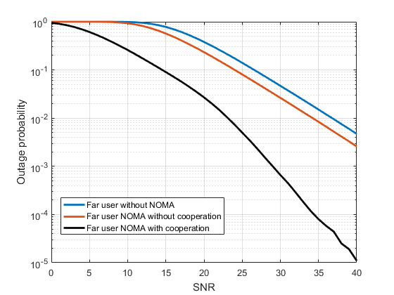
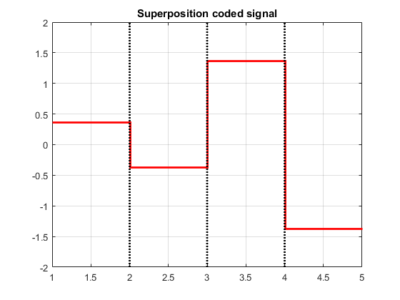
What is cooperative communication? Next post: How to do power allocation in NOMA? We know that NOMA involves successive interference cancellation (SIC) , where one user decodes the message of the other user, from the superposition coded received signal, before decoding his own message. Specifically, the near user decodes the information of the far user while performing SIC. There is no escaping this step. The near user must decode the far user's data anyway. Now that the near user has far user's data, he may as well relay that information to the far user to aid him. Since the far user has a poor channel with the transmitting base station (BS), the retransmission of his data by the near user will provide him diversity. That is, he will receive two different copies of the same message. One from the base station, and one from the near user who is acting like a relay. Thus, we can expect the outage probability of far user to decrease. This concept is called cooperat

Next post: How does user cooperation help NOMA? Till now, we simulated various performance parameters like bit error rate (BER), capacity and outage probability of NOMA by using fixed power allocation method. By fixed power allocation, we mean that regardless of the channel condition, we always set $\alpha_1 = 0.75$ (for far user) and $\alpha_2 = 0.25$ (for near user). This is one way to allocate power. And the advantages of this fixed power allocation method are: No computation required No knowledge of channel state information (CSI) is required But this is not the optimum way to allocate power. If we write a simple MATLAB code to plot the BER as a function of power allocation coefficients, we get a plot like this: ( Download the code here ) Some notes about this plot In this plot, we consider user 1 to be the far user and user 2 to be the near user. Also, we have used fixed power allocation method. That is, we did not alter the coefficients based on channel conditi

Next post: Does power allocation affect NOMA? We saw how to simulate a two user downlink non orthogonal multiple access (NOMA) system in the previous post . There, we plotted the capacity, outage probability and bit error rate (BER) of NOMA by MATLAB simulation. In doing so, we assumed the case of perfect successive interference cancellation (SIC). But in reality, it is not always possible to carry out SIC perfectly. That is, we have an imperfect SIC scenario. A quick look at system model & notation Before looking into what imperfect SIC is, let's take a look at the network model that we are going to use. This is how our network is going to look like. We have a downlink NOMA network with two users. The base station (BS) has two separate messages to transmit to each user. User 1 is the far user/weak user and, user 2 is the near user/strong user. As a quick refresher, remember that the received signals at the far user ($y_1$) and near user ($y_2$) can be repres

Simulation of BER of Non orthogonal multiple access (NOMA) in Rayleigh fading channel - MATLAB code with explanation Next post: What happens when SIC is imperfect? In the previous post , we saw how to simulate a simple two user NOMA network over an AWGN channel in MATLAB. We also plotted the BER vs SNR graphs of both the users and observed the waterfall trend. The AWGN assumption simplified the channel model and allowed us to learn the basic skeletal operation of NOMA. In this post, we will use MATLAB to simulate the capacity, outage and BER performance of a two user NOMA network by following a more realistic model namely, Rayleigh fading model. The MATLAB code to plot BER, capacity and outage probability of NOMA are also available for download in this page . So, let's get started! Wireless channel is prone to multipath propagation and fading. Several channel models are available to capture the effects of fading. Each model deals with a particular scenario.

Simulation of BER of Non orthogonal multiple access (NOMA) in AWGN channel - MATLAB code with explanation You can download the MATLAB code directly here . In the previous two posts, we took a toy example to understand the concept of NOMA and to prove to ourselves that NOMA indeed works as expected. As we said before, NOMA uses superposition coding at the transmitter end and successive interference cancellation at the receiver end. In this post, we will see how to simulate a simple two user NOMA system using MATLAB. We will be plotting the BER performance of NOMA in an additive white gaussian noise (AWGN) channel. The AWGN assumption here is made to keep things simple so that we can pay more attention to the actual skeleton of NOMA implementation. We will improve on this model and do the similar exercise over a Rayleigh fading channel in the next post . The MATLAB code used in this example is available for download here . See this post on How to do power allocation i

NOMA uses power domain multiplexing of users sharing same time and frequency resources. This is accomplished by performing superposition coding at the transmitter and successive interference cancellation (SIC) at the receiver. In the previous post , we saw a graphical view of superposition coding. In this post, we will see how SIC is carried out to decode the superposition coded signal at the receiver side. As a quick recap, we had two users with data x 1 and x 2 respectively. ( What if we had more than two users? ) We first did BPSK modulation to both x 1 and x 2 . Then we obtained the superposition coded signal as x = √a 1 x 1 + √a 2 x 2 where, a 1 and a 2 are the power weights given to x 1 and x 2 respectively, such that, a 1 + a 2 = 1. We took an example of x 1 = 1010 and x 2 = 0110. After BPSK modulation and choosing a 1 = 0.75 and a 2 = 0.25, we obtained the superposition coded signal x, as shown below: Before decoding, let us take a look at SIC al

We have laid the foundation for calculation of carrier concentration in our previous post . In this section, let us solve a simple problem. #1. A silicon pn junction employs the following doping levels. N_A = 10^{17}/cm^3 and N_D = 4\times10^{16}/cm^3 . Determine the hole and electron concentration on the two sides. Solution To solve this problem all you need to know is tabulated below. Type of semiconductor Majority carrier conc. Minority carrier conc. p-type p_p=N_A n_p=\dfrac{n_i^2}{N_A} n-type n_n=N_D p_n=\dfrac{n_i^2}{N_D} where, n_i=1.5\times10^{10}/cm^3 Given data, N_A = 10^{17}/cm^3 N_D = 4\times10^{16}/cm^3 For p-side, Hole (Majority carrier) concentration = p_p=N_A = 10^{17}/cm^3 . Free electron (Minority carrier) concentration = n_p=\dfrac{n_i^2}{N_A} = \dfrac{(1.5\times10^{10})^2}{10^{17}}=2250/cm^3 . For n-side, Free electron (Majority carrier) concentration = n_n=N_D = 4\times10^{16}/cm^3 . Ho

An intrinsic or pure semiconductor (eg., pure Silicon) is an insulator at T=0K. This is because all electrons are bound to their atoms and no free electron is available for conduction. At higher temperatures (T>0K), for example, at room temperature(T=300K), some electrons gain enough thermal energy to break their bonds, cross the band gap energy and enter the conduction band. These electrons are free to conduct current. Free electrons and holes are always generated in pairs. So, for every free electron in the conduction band, there is a hole in the valance band. Let us denote the free electron concentration by n and free hole concentration by p . Since free electrons and holes are generated in pairs, we can say, n=p=n_i where n_i is called intrinsic carrier concentration.Also, np=n_i^2 Typically, number of free electrons in an intrinsic Si at room temperature is of the order of 10 10 /cm 3 . But the number of Si atoms per cm 3 is of the order of 10 22 . Comparing the